z = 0 is a level set specification
of a horizontal plane through the origin.
A vertex may lie on multiple constraints, but the constraints should be non-degenerate, i.e. their gradients should be linearly independent. In particular, the number of constraints cannot exceed the number of dimensions of the ambient space.
For any vertex on level-set constraints, the vertex is projected to the constraint using a Newton-Raphson method any time the vertex is moved. Recall that Newton-Raphson moves along the gradient(s) using a linear approximation to where it estimates the level set to be. It may take multiple iterations of Newton-Raphson to get sufficiently close to the desired level set, and Evolver will complain if things are bad enough that 10 iterations are not enough. Also, in computing the gradient descent motion, the force on a vertex is projected tangent to the constraint before the vertex is moved, to minimize the amount of Newton-Raphson projection needed after motion.
The online documentation for level-set constraints is here.
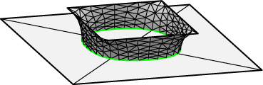
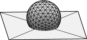
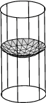
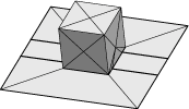
 This example is a soap film between a fixed square wire frame and
a free boundary on a horizontal plane at z = 0 (the green line in
the image). The constraint is
defined in the top part of the datafile, and then applied to the
appropriate vertices and edges. Here are relevant lines from the datafile
free_bdry.fe:
This example is a soap film between a fixed square wire frame and
a free boundary on a horizontal plane at z = 0 (the green line in
the image). The constraint is
defined in the top part of the datafile, and then applied to the
appropriate vertices and edges. Here are relevant lines from the datafile
free_bdry.fe:
constraint 1  // the plane
formula: z = 0

vertices
...
// the contact line on the plane
5   0 0 0 constraint 1
6   1 0 0 constraint 1
7   1 1 0 constraint 1
8   0 1 0 constraint 1
...

edges
...
// the contact line
5  5 6 constraint 1 color green
6  6 7 constraint 1 color green
7  7 8 constraint 1 color green
8  8 5 constraint 1 color green
...
Constraints can be numbered or named; naming is a recent feature, and I still instinctively use numbers. The formula for the level set can be given either as equality of two arbitrary formulas, left side = right side, or as one formula taken to be equal to 0.
Run free_bdry.fe in Evolver. Try this evolution:
g 5
refine edge where on_constraint 1
g 5
r
g 10
u
V
g 10
r
g 10
u
V
u
V
g 100
Note that the surface meets the plane at right angles. This is the consequence of minimizing area with a free boundary, and does not depend on the constraint being flat. However, a flat constraint can be viewed as a symmetry plane for a larger surface. Cutting down a symmetric surface to a smaller piece bounded by mirror planes is a good way to simplify surfaces and speed up evolution. In fact, this surface still has 8-fold symmetry left; can you see how additional symmetry planes could be used to cut the surface down to 1/8 of what is pictured?
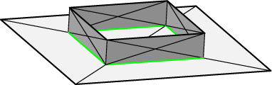
 The simplest way to construct this system is to take the cube example
put its bottom face on a z = 0 constraint, and vary the surface tension
of the bottom face to control the contact angle. This is done in the
datafile moundfull.fe; the bottom face, its
four edges, and its four vertices are all placed on constraint 1. It is
important to remember to place appropriate facets and edges on constraints,
so when you refine them, the newly created vertices will inherit the
appropriate constraints.
The simplest way to construct this system is to take the cube example
put its bottom face on a z = 0 constraint, and vary the surface tension
of the bottom face to control the contact angle. This is done in the
datafile moundfull.fe; the bottom face, its
four edges, and its four vertices are all placed on constraint 1. It is
important to remember to place appropriate facets and edges on constraints,
so when you refine them, the newly created vertices will inherit the
appropriate constraints.
You should now run moundfull.fe in Evolver.
Evolving with 90 degree contact angle: This corresponds to zero surface tension of the interface, so you want to set the tension attribute of the interface facets to 0. Give this command to do so:
set facet tension 0 where on_constraint 1 g 5 refine edge where on_constraint 1 g 5 r g 20 r g 100Evolving with 60 degree contact angle: Don't bother to restart, just change the tension of the interface to -cos(60) and evolve:
  set facet tension -0.5 where on_constraint 1
  g 100
  set facet tension 0.5 where on_constraint 1
  g 100
There are better ways to deal with contact surfaces, but to understand them, we must discuss some details about how Evolver calculates volumes.
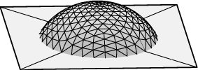
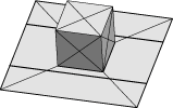
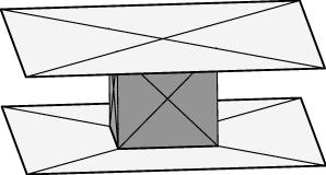
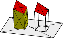 Evolver knows surfaces. Evolver only knows bodies by the surfaces
enclosing them. So Evolver has to calculate the volume of a body
from surface information only. The volume of a body is calculated
by calculating for each facet the oriented volume of the vertical prism
between the facet and the z = 0 plane, and adding the contributions of
all the facets of the body. The orientation of the facet with respect to
the body is taken into account (which is why facets are signed in the
body defintion in the datafile), so facets on the top side of the body
add volume and facets on the bottom subtract. One implication of this
method is that certain types of facet contribute zero to the volume
calculation: horizontal facets at z = 0 and vertical facets. So in the
picture at right, the two bodies have exactly the same calculated volume,
even though the right body is defined only with four facets (just the top
red facets). This image is from the datafile volume.fe, if you want to
run it and look at it from various angles.
Evolver knows surfaces. Evolver only knows bodies by the surfaces
enclosing them. So Evolver has to calculate the volume of a body
from surface information only. The volume of a body is calculated
by calculating for each facet the oriented volume of the vertical prism
between the facet and the z = 0 plane, and adding the contributions of
all the facets of the body. The orientation of the facet with respect to
the body is taken into account (which is why facets are signed in the
body defintion in the datafile), so facets on the top side of the body
add volume and facets on the bottom subtract. One implication of this
method is that certain types of facet contribute zero to the volume
calculation: horizontal facets at z = 0 and vertical facets. So in the
picture at right, the two bodies have exactly the same calculated volume,
even though the right body is defined only with four facets (just the top
red facets). This image is from the datafile volume.fe, if you want to
run it and look at it from various angles.
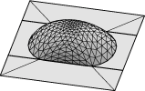
The message here is that bodies do not have to be completely enclosed by facets, and you are free to omit facets that do not contribute to the volume. In particular, you could omit the interface facets from the mound model and still get correct volume calculations. But how about the energy those facets represent?
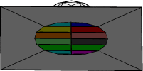 To compensate for the energy represented by missing facets, it is possible
to add an energy defined as the line integral of a vectorfield around
the contact line. Green's Theorem ensures that there is a vectorfield
such that integrating around a boundary curve is equal to the area
integral of the enclosed region. For example, in a horizontal plane,
integrating x dy counterclockwise around the boundary of a region gives
the area of the region. Instead of remembering the formula for Green's
Theorem, you can think of this integral as dividing the area up into
strips of width dy from the y-axis to the curve, so each edge corresponds
to a strip of length x and width dy. The image at right illustrates
how each edge corresponds to a strip.
To compensate for the energy represented by missing facets, it is possible
to add an energy defined as the line integral of a vectorfield around
the contact line. Green's Theorem ensures that there is a vectorfield
such that integrating around a boundary curve is equal to the area
integral of the enclosed region. For example, in a horizontal plane,
integrating x dy counterclockwise around the boundary of a region gives
the area of the region. Instead of remembering the formula for Green's
Theorem, you can think of this integral as dividing the area up into
strips of width dy from the y-axis to the curve, so each edge corresponds
to a strip of length x and width dy. The image at right illustrates
how each edge corresponds to a strip.
A constraint definition can have an "energy" integrand added to it, which means that this integrand will be integrated along every edge on the constraint and the result added to the total energy of the surface. The datafile mound.fe is suitably modified, with the constraint definition thus:
parameter angle = 90    // interior angle between plane and surface, degrees

#define PLANET  (-cos(angle*pi/180))  // virtual tension of facet on plane

constraint 1   /* the table top */
formula: z = 0
energy:  // for contact angle
e1: 0
e2: PLANET*x
e3: 0
Try running mound.fe with the same evolution as above for moundful.fe, and you will see there is no problem with a shrinking contact line. NOTE: To change the contact angle now, you change the
angle
variable,
angle := 60and so forth.
Further benefits of replacing facets with constraint integrals are less memory use and faster calculation. Also, integrand formulas can contain variables, so changing one variable such as "angle" automatically changes the energy.
NOTE: Be careful with the orientation of your edges. The integrand is evaluated along the orientation you give in the datafile. Remember that Evolver does NOT know the orientation of this edge relative to the area you are omitting!!
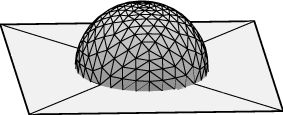
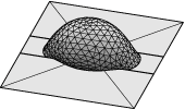
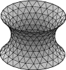
 Constraint energy integrals are very useful with curved constraints,
which are awkward to cover with flat triangles. At right is shown
the top surface of liquid in a vertical tube, with the liquid making
a 45 degree contact angle with the wall. This time, the constraint
integrand gives the area of the tube below the contact line, with each
edge of the contact line accounting for the tube wall directly below it:
Constraint energy integrals are very useful with curved constraints,
which are awkward to cover with flat triangles. At right is shown
the top surface of liquid in a vertical tube, with the liquid making
a 45 degree contact angle with the wall. This time, the constraint
integrand gives the area of the tube below the contact line, with each
edge of the contact line accounting for the tube wall directly below it:
parameter radius = 1  // of tube
parameter height = 4  // of tube
parameter angle = 45  // interior contact angle, degrees

#define WALLT (-cos(angle*pi/180))

constraint 1  // the tube wall, for contact line
formula: x^2 + y^2 = radius^2
energy:
e1:  -WALLT*z*y/radius
e2:   WALLT*z*x/radius
e3:   0
The full datafile is capillary.fe. Run it in Evolver with this evolution:
 r
 g 5
 r
 g 10
Looks pretty good. Now try a further g 50. You should see a problem with the edges along the contact line getting very uneven. This is a general problem with curved constraints, and is not caused by using constraint integrals. Even though the constraint the edges are on is curved, the edges themselves are still straight, and opening gaps between the edges and the constraint often turns out to save energy. The next section shows a way to prevent this.
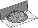
parameter flute_count = 3   // start with 3 planes, enough for 6 vertices
constraint 3
formula:  sin(flute_count*atan2(y,x))
The revised datafile is capillary2.fe. If you run this, you will find no problems with edges shortcutting the curved wall. NOTE: the flute_count variable has to be doubled each refinement to provide enough planes for the vertices. I have made that automatic in this datafile by re-defining the
r command in
the bottom section of the datafile:
r :::= { flute_count *= 2; 'r' }
The :::= is syntax just for re-defining single-letter commands,
and the single quotes around r on the right mean use the original meaning of r.
 The example shown at right is a drop confined to lie on a wettable
strip, where its contact angle is 60 degrees. Here are relevant parts
of the datafile, moundpad.fe:
The example shown at right is a drop confined to lie on a wettable
strip, where its contact angle is 60 degrees. Here are relevant parts
of the datafile, moundpad.fe:
parameter angle = 60    // interior angle between plane and surface, degrees
parameter xleft = -.2   // left side of wettable strip
parameter xright = 1.2  // right side of wettable strip

#define LOWERT  (-cos(angle*pi/180))  // virtual tension of facet on plane

constraint 1   /* the table top */
formula: z = 0
energy:  // for contact angle
e1: -(LOWERT*y)
e2: 0
e3: 0

constraint leftcon nonnegative
formula: x - xleft

constraint rightcon nonpositive
formula: x - xright

vertices
1   0.0  0.0 0.0  constraint 1,leftcon,rightcon  /* 4 vertices on plane */
2   1.0  0.0 0.0  constraint 1,leftcon,rightcon
3   1.0  1.0 0.0  constraint 1,leftcon,rightcon
4   0.0  1.0 0.0  constraint 1,leftcon,rightcon
...
edges
1   1 2    constraint 1,leftcon,rightcon  /* 4 edges on plane */
2   2 3    constraint 1,leftcon,rightcon
3   3 4    constraint 1,leftcon,rightcon
4   4 1    constraint 1,leftcon,rightcon
...
Notice I'm using constraint names here to show how it is done. Also notice that an element can be on multiple one-sided constraints; only the constraints that are actually hit count for the independence requirement.
Run moundpad.fe in Evolver, with the evolution
 refine edge where on_constraint 1
 g 5
 r
 g 10
 r
 g 100
 This is a more elaborate use of one-sided constraints. Here the
droplet is large enough to slop over the wettable strip onto the
relatively nonwettable outside (contact angle 120 degrees).
The variable contact tension can be implemented by using a
conditional expression in the constraint integrand?
This is a more elaborate use of one-sided constraints. Here the
droplet is large enough to slop over the wettable strip onto the
relatively nonwettable outside (contact angle 120 degrees).
The variable contact tension can be implemented by using a
conditional expression in the constraint integrand?
parameter wet_angle = 60    // interior angle between plane and surface, degree
parameter dry_angle = 120   // interior angle outside strip

parameter xleft =  .2   // left side of wettable strip
parameter xright = .8  // right side of wettable strip

#define WETT  (-cos(wet_angle*pi/180))  // virtual tension of facet on plane
#define DRYT  (-cos(dry_angle*pi/180))  // virtual tension of facet on plane

constraint 1   /* the table top */
formula: z = 0
energy:  // For contact angle.  Note that conditional expression is just
         // the two tensions because dx strips each have constant tension!!!!
e1: (x > xleft and x < xright) ? -(WETT*y) : -(DRYT*y)
e2: 0
e3: 0
However, note carefully that the integrand has been set up so the strips
it represents are each of constant tension! If one did dy strips, the
integrand would have to be more elaborate, and when x is outside the wettable
strip, still account exactly for the interface tension inside the strip.
A further feature of this example is the use of multiple one-sided constraints to keep different parts of the contact line in their own regions. There are vertices explicitly constrained to lie on the edges of the wettable strip. The full datafile is moundstrip.fe. An evolution:
g 5
r
u
V
V
g 10
g 20
r
g 100
 Since it is so useful to be able to replace facets with constraint
integrals for energy, I realized it would be good to replace facets
with constraint integrals for computing volumes also. So if one
adds a "content" integrand to a constraint, then this integrand is
integrated along each edge on the constraint, and the result added
to the volume of adjacent bodies, according to the relative orientation
of the edge and the body.
Unfortunately (in the view of some people),
this works out as if you were doing Green's Theorem with the boundary
oriented clockwise around the missing region instead of counterclockwise.
But that choice seemed natural when I first programmed it in, and once
something like that gets in, it can't be changed without breaking a
lot of datafiles for a lot of people. So check and double-check that
you are getting the proper results.
Since it is so useful to be able to replace facets with constraint
integrals for energy, I realized it would be good to replace facets
with constraint integrals for computing volumes also. So if one
adds a "content" integrand to a constraint, then this integrand is
integrated along each edge on the constraint, and the result added
to the volume of adjacent bodies, according to the relative orientation
of the edge and the body.
Unfortunately (in the view of some people),
this works out as if you were doing Green's Theorem with the boundary
oriented clockwise around the missing region instead of counterclockwise.
But that choice seemed natural when I first programmed it in, and once
something like that gets in, it can't be changed without breaking a
lot of datafiles for a lot of people. So check and double-check that
you are getting the proper results.
I use the word "content" instead of "volume" since this method also applies to area in the string model, with suitable modifications.
An example of a constraint content integral is the datafile plates_column.fe, which is a liquid column between two parallel plates, with the endcap facets omitted (the large squares are just for display, they are not part of the body definition). Relevant parts of the datafile:
parameter top_angle = 70    // interior angle between plane and surface, degrees
parameter bottom_angle = 70 // interior angle between plane and surface, degrees
parameter height = 1    // separation of plates

// Contact surface tensions
#define UPPERT  (-cos(top_angle*pi/180))  // virtual tension of facet on plane
#define LOWERT (-cos(bottom_angle*pi/180))

constraint 1   /* the lower plate */
formula: z = 0
energy:  // for contact angle
e1: -(LOWERT*y)
e2: 0
e3: 0
constraint 2   /* the upper plate */
formula: z = height
energy:  // for contact angle and gravitational energy under missing facets
e1: -(UPPERT*y) + G*z^2/2*y
e2: 0
e3: 0
content:
c1: z*y
c2: 0
c3: 0
NOTE: When setting up a content integral, always carefully check when you load the file in Evolver that the volume is correct. It is very easy to get the sign wrong. On the plus side, since Evolver does know the orientation of edges relative to bodies, the edges don't all have to have a consistent orientation.
 Construct a datafile for a drop of liquid that sits at the junction
of a horizontal plane and a vertical wall, with contact angle 110 degrees
on the wall and 60 degrees on the plane. Construct one datafile using
full facets around the drop, and construct a second datafile using
constraint integrals to replace the facets on the plane and wall.
Use the first datafile to check the second; when you load them, they
should have identical energy.
Construct a datafile for a drop of liquid that sits at the junction
of a horizontal plane and a vertical wall, with contact angle 110 degrees
on the wall and 60 degrees on the plane. Construct one datafile using
full facets around the drop, and construct a second datafile using
constraint integrals to replace the facets on the plane and wall.
Use the first datafile to check the second; when you load them, they
should have identical energy.